本篇程序主要参考:
- 准一维方格子能带图(附Python代码)
- 佩尔斯替换 Peierls substitution
- 方格子的霍夫斯塔特蝴蝶(附Python代码)
- 陈数Chern number的计算(高效法,附Python/Matlab代码)
- 多端体系的量子输运(附Python代码)
- 介观体系中的Landauer–Büttiker公式
- Python开源项目Guan
本篇代码目录:
- 二维方格子朗道能级和陈数/霍尔电导
- 通过六端口的量子输运计算方格子在磁场下的霍尔电导
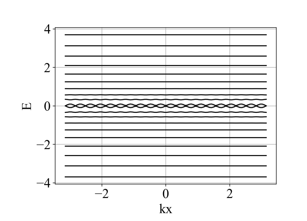
1. 二维方格子朗道能级和陈数/霍尔电导
"""
This code is supported by the website: https://www.guanjihuan.com
The newest version of this code is on the web page: https://www.guanjihuan.com/archives/18306
"""

import numpy as np
from math import *
import cmath
import functools
import guan

def hamiltonian(kx, ky, Ny, B):
    h00 = np.zeros((Ny, Ny), dtype=complex)
    h01 = np.zeros((Ny, Ny), dtype=complex)
    t = 1
    for iy in range(Ny-1):
        h00[iy, iy+1] = t
        h00[iy+1, iy] = t
    h00[Ny-1, 0] = t*cmath.exp(1j*ky)
    h00[0, Ny-1] = t*cmath.exp(-1j*ky)
    for iy in range(Ny):
        h01[iy, iy] = t*cmath.exp(-2*np.pi*1j*B*iy)
    matrix = h00 + h01*cmath.exp(1j*kx) + h01.transpose().conj()*cmath.exp(-1j*kx)
    return matrix


def main():
    Ny = 21

    k_array = np.linspace(-pi, pi, 100)
    H_k = functools.partial(hamiltonian, ky=0, Ny=Ny, B=1/Ny)
    eigenvalue_array = guan.calculate_eigenvalue_with_one_parameter(k_array, H_k)
    guan.plot(k_array, eigenvalue_array, xlabel='kx', ylabel='E', style='k')

    H_k = functools.partial(hamiltonian, Ny=Ny, B=1/Ny)
    chern_number = guan.calculate_chern_number_for_square_lattice_with_efficient_method(H_k, precision=100)
    print(chern_number)
    print(sum(chern_number))


if __name__ == '__main__':
    main()
当Ny=20时,运行结果:
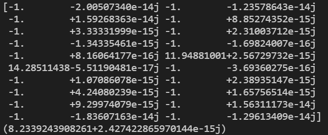
说明:这里计算结果不正确,把所有能带的陈数相加,结果不为零。是因为中间能带部分交叉简并导致的错误。关于简并能带的陈数计算,参考这篇:陈数Chern number的计算(多条能带的Wilson loop方法,附Python代码)。
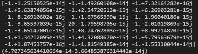
如果把Ny取为21(奇数),能带不存在部分交叉简并,计算结果正确。运算结果为:

2. 通过六端口的量子输运计算方格子在磁场下的霍尔电导
"""
This code is supported by the website: https://www.guanjihuan.com
The newest version of this code is on the web page: https://www.guanjihuan.com/archives/18306
"""
import numpy as np
import time
import cmath
import guan
def get_lead_h00(width):
h00 = np.zeros((width, width))
for i0 in range(width-1):
h00[i0, i0+1] = 1
h00[i0+1, i0] = 1
return h00
def get_lead_h01(width):
h01 = np.identity(width)
return h01
def get_center_hamiltonian(Nx, Ny, B):
h = np.zeros((Nx*Ny, Nx*Ny), dtype=complex)
for x0 in range(Nx-1):
for y0 in range(Ny):
h[x0*Ny+y0, (x0+1)*Ny+y0] = 1*cmath.exp(-2*np.pi*1j*B*y0) # x方向的跃迁
h[(x0+1)*Ny+y0, x0*Ny+y0] = 1*cmath.exp(2*np.pi*1j*B*y0)
for x0 in range(Nx):
for y0 in range(Ny-1):
h[x0*Ny+y0, x0*Ny+y0+1] = 1 # y方向的跃迁
h[x0*Ny+y0+1, x0*Ny+y0] = 1
return h
def main():
start_time = time.time()
width = 21
length = 72
fermi_energy_array = np.arange(-4, 4, .05)
# 中心区的哈密顿量
H_cetner = get_center_hamiltonian(Nx=length, Ny=width, B=1/width)
# 电极的h00和h01
lead_h00 = get_lead_h00(width)
lead_h01 = get_lead_h01(width)
transmission_12_array = []
transmission_13_array = []
transmission_14_array = []
transmission_15_array = []
transmission_16_array = []
transmission_1_all_array = []
for fermi_energy in fermi_energy_array:
print(fermi_energy)
# 几何形状如下所示:
# lead2 lead3
# lead1(L) lead4(R)
# lead6 lead5
# 电极到中心区的跃迁矩阵
h_lead1_to_center = np.zeros((width, width*length), dtype=complex)
h_lead2_to_center = np.zeros((width, width*length), dtype=complex)
h_lead3_to_center = np.zeros((width, width*length), dtype=complex)
h_lead4_to_center = np.zeros((width, width*length), dtype=complex)
h_lead5_to_center = np.zeros((width, width*length), dtype=complex)
h_lead6_to_center = np.zeros((width, width*length), dtype=complex)
move = 10 # the step of leads 2,3,6,5 moving to center
for i0 in range(width):
h_lead1_to_center[i0, i0] = 1
h_lead2_to_center[i0, width*(move+i0)+(width-1)] = 1
h_lead3_to_center[i0, width*(length-move-1-i0)+(width-1)] = 1
h_lead4_to_center[i0, width*(length-1)+i0] = 1
h_lead5_to_center[i0, width*(length-move-1-i0)+0] = 1
h_lead6_to_center[i0, width*(i0+move)+0] = 1
# 自能
self_energy1, gamma1 = guan.self_energy_of_lead_with_h_lead_to_center(fermi_energy, lead_h00, lead_h01, h_lead1_to_center)
self_energy2, gamma2 = guan.self_energy_of_lead_with_h_lead_to_center(fermi_energy, lead_h00, lead_h01, h_lead2_to_center)
self_energy3, gamma3 = guan.self_energy_of_lead_with_h_lead_to_center(fermi_energy, lead_h00, lead_h01, h_lead3_to_center)
self_energy4, gamma4 = guan.self_energy_of_lead_with_h_lead_to_center(fermi_energy, lead_h00, lead_h01, h_lead4_to_center)
self_energy5, gamma5 = guan.self_energy_of_lead_with_h_lead_to_center(fermi_energy, lead_h00, lead_h01, h_lead5_to_center)
self_energy6, gamma6 = guan.self_energy_of_lead_with_h_lead_to_center(fermi_energy, lead_h00, lead_h01, h_lead6_to_center)
# 整体格林函数
green = np.linalg.inv(fermi_energy*np.eye(width*length)-H_cetner-self_energy1-self_energy2-self_energy3-self_energy4-self_energy5-self_energy6)
# Transmission
transmission_12 = np.trace(np.dot(np.dot(np.dot(gamma1, green), gamma2), green.transpose().conj()))
transmission_13 = np.trace(np.dot(np.dot(np.dot(gamma1, green), gamma3), green.transpose().conj()))
transmission_14 = np.trace(np.dot(np.dot(np.dot(gamma1, green), gamma4), green.transpose().conj()))
transmission_15 = np.trace(np.dot(np.dot(np.dot(gamma1, green), gamma5), green.transpose().conj()))
transmission_16 = np.trace(np.dot(np.dot(np.dot(gamma1, green), gamma6), green.transpose().conj()))
transmission_12_array.append(np.real(transmission_12))
transmission_13_array.append(np.real(transmission_13))
transmission_14_array.append(np.real(transmission_14))
transmission_15_array.append(np.real(transmission_15))
transmission_16_array.append(np.real(transmission_16))
transmission_1_all_array.append(np.real(transmission_12+transmission_13+transmission_14+transmission_15+transmission_16))
guan.plot(fermi_energy_array, transmission_12_array, xlabel='Fermi energy', ylabel='Transmission_12')
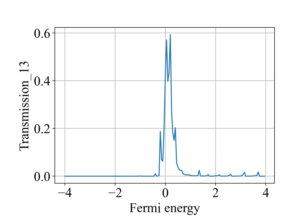
guan.plot(fermi_energy_array, transmission_13_array, xlabel='Fermi energy', ylabel='Transmission_13')
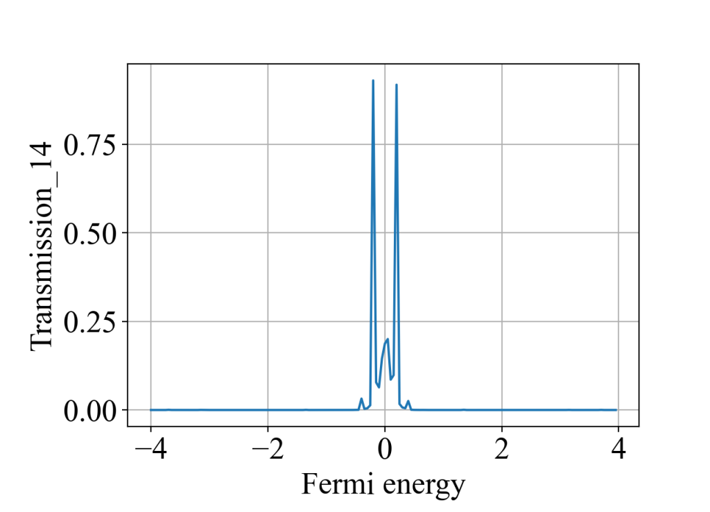
guan.plot(fermi_energy_array, transmission_14_array, xlabel='Fermi energy', ylabel='Transmission_14')
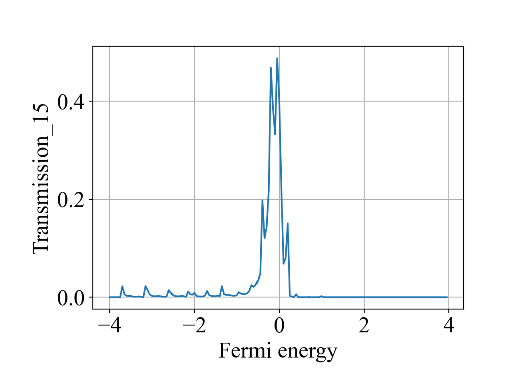
guan.plot(fermi_energy_array, transmission_15_array, xlabel='Fermi energy', ylabel='Transmission_15')
guan.plot(fermi_energy_array, transmission_16_array, xlabel='Fermi energy', ylabel='Transmission_16')
guan.plot(fermi_energy_array, transmission_1_all_array, xlabel='Fermi energy', ylabel='Transmission_1_all')
end_time = time.time()
print('运行时间=', end_time-start_time)
if __name__ == '__main__':
main()运行结果:
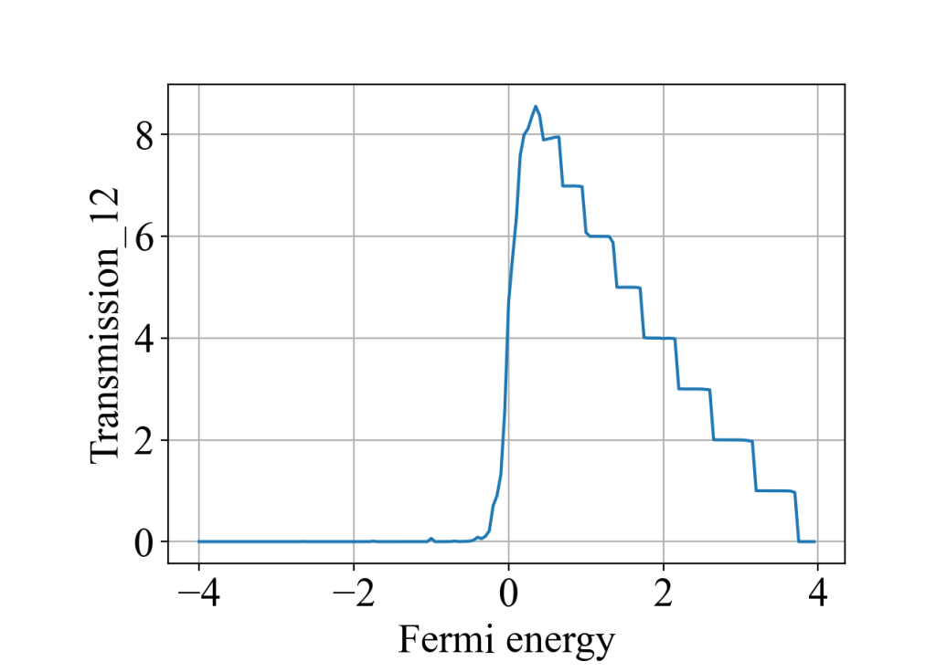
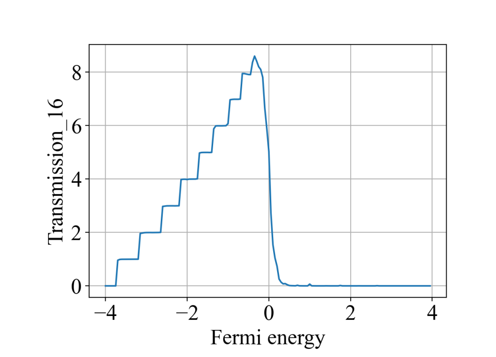

说明1:电极2,3,6,5需要往中间移一点,即move>0,否则相邻电极会相互接触,计算结果出现不了明显的平台。
说明2:对于方格子的情况,通过陈数计算的霍尔电导和通过六端输运计算的霍尔电导在数值上无法完全对应上,这可能是由于前者算的是二维体系,后者算的是准一维体系,存在一定的散射。但总体趋势是一致的:费米能越接近0,霍尔电导值越大,且呈现台阶状。
更多参考资料:
[1] B. Andrei Bernevig - Topological Insulators and Topological Superconductors
[2] A. H. MacDonald - Landau-level subband structure of electrons on a square lattice
[3] Quantized Hall Conductance in a Two-Dimensional Periodic Potential
[4] Route towards Localization for Quantum Anomalous Hall Systems with Chern Number 2
[5] Localization trajectory and Chern-Simons axion coupling for bilayer quantum anomalous Hall systems
【说明:本站主要是个人笔记和代码的分享,内容可能会不定期修改。目前文章支持直接转载,引用或转载请注明出处:https://www.guanjihuan.com 。本站采用知识共享署名许可协议 CC BY】
你好,请问那个算出来的霍尔电导[(ohm*cm)^-1]和陈数(e^2/h)之间是怎么换算的呢?这两个之间不是相差了一个1/cm的关系吗。我是用wannier90算了一个具体材料的反常霍尔电导[(ohm*cm)^-1],但是不知道怎么换算成(e^2/h)。我看到很多文献里面,霍尔电导[(ohm*cm)^-1]-E(eV)和C(e^2/h)-E(eV)的关系图是看起来一样的,感觉就只相差了一个常系数,有点不太理解?(对不起,我的理论基础真的太差了)
霍尔电导和陈数的关系就是差了这么一个系数,证明过程是从 Kubo 公式出发,可以参考这篇:1982 - Thouless et al. - Quantized Hall Conductance in a Two-Dimensional Periodic Potential。所以陈数一般也叫做 TKNN 数,由这篇文章的作者名字的首字母组成。
万分感谢
嗯,都是可以的,不影响能带和物理结果。
请问二维方格子朗道能级和陈数/霍尔电导这段代码中的哈密顿量用的是晶格规范吗?
这里的哈密顿量相当于沿着y方向扩了Ny倍胞的哈密顿量,设原晶格常数(扩胞前)为1,那么h00[Ny-1, 0] = t*cmath.exp(1j*ky)这里指数上是ky的原因是不是因为在周期边界条件下,第Ny-1个格点和第0个格点之间差了原晶格常数1的距离吗?
嗯,是这样的。这样的布里渊区的ky范围就是在-pi到pi。
你好,我想问下为什么kx取值还是-pi到pi,不应该除以Ny吗?还有就是h00[Ny-1, 0] = t*cmath.exp(1j*ky)这里指数上应该是Ny*ky吧?
我把晶格常数(也就是元胞)的宽度取为1,而不是原子间距,所以这里布里渊区的范围保持不变。
你这个做法也是对的,如果指数上是Ny*ky,那么布里渊区的范围是要除以Ny。