非平衡格林函数计算电导（附Python代码）

准一维的方格子哈密顿量（以宽度3为例）为

在上面最后的表达式中，第一项是H00，表示的是元胞内部的哈密顿量矩阵；第二项是H01，表示的是元胞间的跃迁矩阵。

1. 给出全部算法的代码

这里给出“用非平衡格林函数计算准一维方格子电导”的Python代码，相关公式见参考资料。其中用到戴森方程，格林函数公式参考这篇：使用Dyson方程迭代方法计算态密度（附Python代码）。

"""
This code is supported by the website: https://www.guanjihuan.com
The newest version of this code is on the web page: https://www.guanjihuan.com/archives/948
"""

import numpy as np
import matplotlib.pyplot as plt
import copy
import time


def matrix_00(width=10):  # 不赋值时默认为10
    h00 = np.zeros((width, width))
    for width0 in range(width-1):
        h00[width0, width0+1] = 1
        h00[width0+1, width0] = 1
    return h00


def matrix_01(width=10):  # 不赋值时默认为10
    h01 = np.identity(width)
    return h01


def main():
    start_time = time.time()
    h00 = matrix_00(width=5)
    h01 = matrix_01(width=5)
    fermi_energy_array = np.arange(-4, 4, .01)
    plot_conductance_energy(fermi_energy_array, h00, h01)
    end_time = time.time()
    print('运行时间=', end_time-start_time)


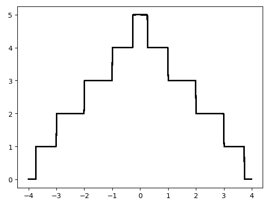
def plot_conductance_energy(fermi_energy_array, h00, h01):  # 画电导与费米能关系图
    dim = fermi_energy_array.shape[0]
    cond = np.zeros(dim)
    i0 = 0
    for fermi_energy0 in fermi_energy_array:
        cond0 = np.real(conductance(fermi_energy0 + 1e-12j, h00, h01))
        cond[i0] = cond0
        i0 += 1
    plt.plot(fermi_energy_array, cond, '-k')
    plt.show()


def transfer_matrix(fermi_energy, h00, h01, dim):   # 转移矩阵T。dim是传递矩阵h00和h01的维度
    transfer = np.zeros((2*dim, 2*dim), dtype=complex)
    transfer[0:dim, 0:dim] = np.dot(np.linalg.inv(h01), fermi_energy*np.identity(dim)-h00)   # np.dot()等效于np.matmul()
    transfer[0:dim, dim:2*dim] = np.dot(-1*np.linalg.inv(h01), h01.transpose().conj())
    transfer[dim:2*dim, 0:dim] = np.identity(dim)
    transfer[dim:2*dim, dim:2*dim] = 0  # a:b代表 a <= x < b，左闭右开
    return transfer  # 返回转移矩阵


def green_function_lead(fermi_energy, h00, h01, dim):  # 电极的表面格林函数
    transfer = transfer_matrix(fermi_energy, h00, h01, dim)
    eigenvalue, eigenvector = np.linalg.eig(transfer)
    ind = np.argsort(np.abs(eigenvalue))
    temp = np.zeros((2*dim, 2*dim), dtype=complex)
    i0 = 0
    for ind0 in ind:
        temp[:, i0] = eigenvector[:, ind0]
        i0 += 1
    s1 = temp[dim:2*dim, 0:dim]
    s2 = temp[0:dim, 0:dim]
    s3 = temp[dim:2*dim, dim:2*dim]
    s4 = temp[0:dim, dim:2*dim]
    right_lead_surface = np.linalg.inv(fermi_energy*np.identity(dim)-h00-np.dot(np.dot(h01, s2), np.linalg.inv(s1)))
    left_lead_surface = np.linalg.inv(fermi_energy*np.identity(dim)-h00-np.dot(np.dot(h01.transpose().conj(), s3), np.linalg.inv(s4)))
    return right_lead_surface, left_lead_surface  # 返回右电极的表面格林函数和左电极的表面格林函数


def self_energy_lead(fermi_energy, h00, h01, dim):  # 电极的自能
    right_lead_surface, left_lead_surface = green_function_lead(fermi_energy, h00, h01, dim)
    right_self_energy = np.dot(np.dot(h01, right_lead_surface), h01.transpose().conj())
    left_self_energy = np.dot(np.dot(h01.transpose().conj(), left_lead_surface), h01)
    return right_self_energy, left_self_energy  # 返回右边电极自能和左边电极自能


def conductance(fermi_energy, h00, h01, nx=300):  # 计算电导
    dim = h00.shape[0]
    right_self_energy, left_self_energy = self_energy_lead(fermi_energy, h00, h01, dim)
    for ix in range(nx):
        if ix == 0:
            green_nn_n = np.linalg.inv(fermi_energy*np.identity(dim)-h00-left_self_energy)
            green_0n_n = copy.deepcopy(green_nn_n)  # 如果直接用等于，两个变量会指向相同的id，改变一个值，另外一个值可能会发生改变，容易出错，所以要用上这个COPY
        elif ix != nx-1:
            green_nn_n = np.linalg.inv(fermi_energy*np.identity(dim)-h00-np.dot(np.dot(h01.transpose().conj(), green_nn_n), h01))
            green_0n_n = np.dot(np.dot(green_0n_n, h01), green_nn_n)
        else:
            green_nn_n = np.linalg.inv(fermi_energy*np.identity(dim)-h00-np.dot(np.dot(h01.transpose().conj(), green_nn_n), h01)-right_self_energy)
            green_0n_n = np.dot(np.dot(green_0n_n, h01), green_nn_n)
    gamma_right = (right_self_energy - right_self_energy.transpose().conj())*(0+1j)
    gamma_left = (left_self_energy - left_self_energy.transpose().conj())*(0+1j)
    transmission = np.trace(np.dot(np.dot(np.dot(gamma_left, green_0n_n), gamma_right), green_0n_n.transpose().conj()))
    return transmission  # 返回电导值


if __name__ == '__main__':
    main()

运行结果：

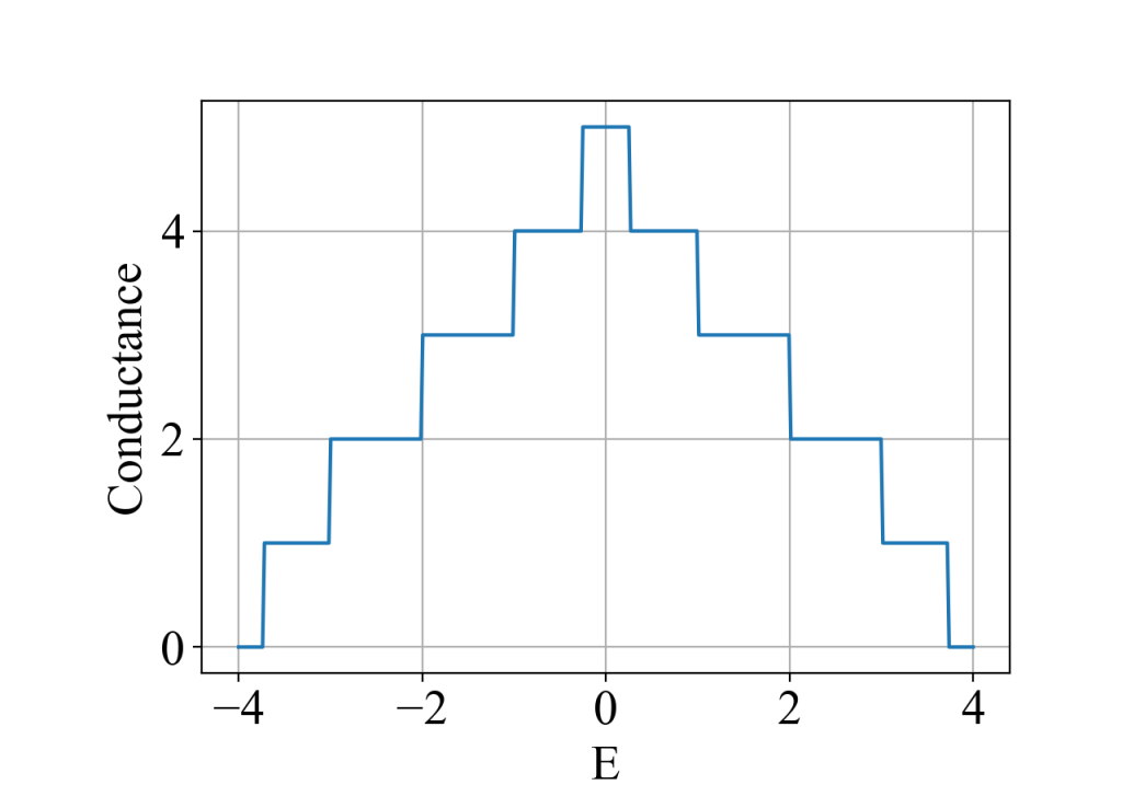
2. 使用Guan软件包

网址：https://py.guanjihuan.com/。

import guan
import numpy as np

fermi_energy_array = np.linspace(-4, 4, 400)
h00 = guan.hamiltonian_of_finite_size_system_along_one_direction(4)
h01 = np.identity(4)
conductance_array = guan.calculate_conductance_with_fermi_energy_array(fermi_energy_array, h00, h01)
guan.plot(fermi_energy_array, conductance_array, xlabel='E', ylabel='Conductance', style='-')

运行结果：

3. 使用Kwant软件包

访问这篇：https://www.guanjihuan.com/archives/2033。

参考文献：

[1] Landauer R. Electrical resistance of disordered one-dimensional lattices. The Philosophical Magazine: A Journal of Theoretical Experimental and Applied Physics, 1970, 21(172):863-867.

[2] Supriyo, Datta. Electronic transport in mesoscopic systems. 世界图书出版公司, 2004.

[3] Lee D H, Joannopoulos J D. Simple scheme for surface-band calculations. I. Phys. Rev. B, 1981, 23:4988-4996.

[4] Lee D, Joannopoulos J. Simple scheme for surface-band calculations. II. The Green’s function. Phys. Rev. B, 1981, 23:4997-5004.

[5] Jintao Zhang, Electronic transport in Z-junction carbon nanotubes, J. Chem. Phys. 120, 7733 (2004).

[6] MacKinnon A. The calculation of transport properties and density of states of disordered solids. Zeitschrift für Physik B Condensed Matter, 1985, 59(4):385-390.

[7] https://www.iue.tuwien.ac.at/phd/karamitaheri/node23.html

[8] https://sundoc.bibliothek.uni-halle.de/diss-online/07/07H039/t5.pdf

以上[8]链接可能已经失效，以下是对应的文件：

6,268 次浏览

【说明：本站主要是个人的一些笔记和代码分享，内容可能会不定期修改。为了使全网显示的始终是最新版本，这里的文章未经同意请勿转载。引用请注明出处：https://www.guanjihuan.com】