定态薛定谔方程为:

一维无限深势阱的势函数定义为:

解析推导(参考教科书),得到归一化的波函数为:

能量本征值为:

本篇使用有限差分的方法,数值求解一维无限深势阱的薛定谔方程。
主要需要处理的是薛定谔方程中二阶导数的离散化 [1]:

Python 代码如下:
"""
This code is supported by the website: https://www.guanjihuan.com
The newest version of this code is on the web page: https://www.guanjihuan.com/archives/47514
"""
import numpy as np
import matplotlib.pyplot as plt
import scipy
plt.rcParams['font.sans-serif'] = ['SimHei'] # 在画图中显示中文
plt.rcParams['axes.unicode_minus'] = False # 显示中文后,加上这个才可以正常显示负号
# 物理常数定义
hbar = 1.0545718e-34 # 约化普朗克常数 (J·s)
m = 9.109e-31 # 电子质量 (kg)
a = 1e-9 # 势阱宽度 1nm (m)
# 解析波函数
def infinite_well_wavefunction(n, x, a):
"""返回第n能级的波函数"""
return np.sqrt(2/a) * np.sin(n * np.pi * x / a)
# 解析能级
def infinite_well_energy(n, a, m, hbar):
"""返回第n能级的能量"""
return (n**2 * np.pi**2 * hbar**2) / (2 * m * a**2)
def solve_infinite_well_numerically(a=1e-9, N=3000, num_states=5):
"""
有限差分数值求解一维无限深势阱的薛定谔方程
参数:
a: 势阱宽度
N: 网格点数
num_states: 要计算的本征态数量
"""
# 离散化参数
x_array = np.linspace(0, a, N)
dx = x_array[1] - x_array[0]
# 构建哈密顿矩阵:二阶导数的离散化(三点中心差分)
coefficient = -hbar**2 / (2 * m)
main_diag = -2 * np.ones(N) * coefficient / dx**2
off_diag = np.ones(N-1) * coefficient / dx**2
H = scipy.sparse.diags([main_diag, off_diag, off_diag], [0, -1, 1], format='csc')
# 对于N=5个网格点的例子:
# H = coefficient/dx² ×
# ⎡ -2 1 0 0 0 ⎤
# ⎢ 1 -2 1 0 0 ⎥
# ⎢ 0 1 -2 1 0 ⎥
# ⎢ 0 0 1 -2 1 ⎥
# ⎣ 0 0 0 1 -2 ⎦
# 求解本征值和本征向量
eigenvalues, eigenvectors = scipy.sparse.linalg.eigs(H, k=num_states, which='SM')
eigenvalues = np.real(eigenvalues)
# 排序本征值和本征向量
idx = eigenvalues.argsort()
eigenvalues = eigenvalues[idx]
eigenvectors = eigenvectors[:, idx]
return x_array, eigenvalues, eigenvectors
# 数值求解
x_array, E_num, psi_num = solve_infinite_well_numerically()
E_num_ev = E_num / 1.602e-19 # J 单位转换为 eV 单位
print("数值求解结果:")
for i, E in enumerate(E_num_ev):
print(f"状态 {i+1}: E = {E:.3f} eV")
print("解析求解结果:")
for i in range(5):
n = i + 1
E_analytical = infinite_well_energy(n, a, m, hbar) / 1.602e-19
error = abs(E_num_ev[i] - E_analytical) / E_analytical * 100
print(f"状态 {i+1}: 解析解 E = {E_analytical:.4f} eV, 数值求解误差 Error = {error:.2f}%")
# 绘制数值求解的能级图
plt.figure(figsize=(8, 6))
for n, E in enumerate(E_num_ev[:6], 1):
plt.axhline(y=E, color='r', linestyle='-', linewidth=2) # 主要的画图命令
plt.text(a*1e9/2, E + 0.1, f'n={n}', ha='center', va='bottom', fontsize=12)
plt.xlabel('势阱位置')
plt.ylabel('能量 (eV)')
plt.title('一维无限深势阱的能级(数值解)')
plt.grid(True, alpha=0.3)
plt.ylim(0, max(E_num_ev[:6]) + 1)
plt.show()
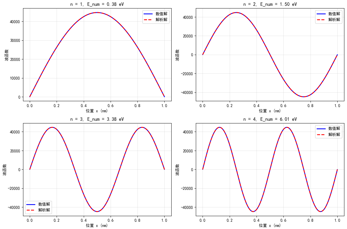
# 绘制数值解与解析解的比较
plt.figure(figsize=(12, 8))
for i in range(4):
# 数值解
psi_numerical = np.real(psi_num[:, i])
norm = np.sqrt(np.trapz(psi_numerical**2, x_array))
psi_numerical /= norm # 归一化数值解
# 确保符号一致(本征向量符号可能任意)
if np.dot(psi_numerical, infinite_well_wavefunction(i+1, x_array, a)) < 0:
psi_numerical *= -1
# 解析解
psi_analytical = infinite_well_wavefunction(i+1, x_array, a)
plt.subplot(2, 2, i+1)
plt.plot(x_array*1e9, psi_numerical, 'b-', label='数值解', linewidth=2)
plt.plot(x_array*1e9, psi_analytical, 'r--', label='解析解', linewidth=2)
plt.xlabel('位置 x (nm)')
plt.ylabel('波函数')
plt.title(f'n = {i+1}, E_num = {E_num_ev[i]:.2f} eV')
plt.legend()
plt.grid(True, alpha=0.3)
plt.tight_layout()
plt.show()运行结果:
数值求解结果:
状态 1: E = 0.376 eV
状态 2: E = 1.502 eV
状态 3: E = 3.380 eV
状态 4: E = 6.009 eV
状态 5: E = 9.390 eV
解析求解结果:
状态 1: 解析解 E = 0.3761 eV, 数值求解误差 Error = 0.13%
状态 2: 解析解 E = 1.5043 eV, 数值求解误差 Error = 0.13%
状态 3: 解析解 E = 3.3848 eV, 数值求解误差 Error = 0.13%
状态 4: 解析解 E = 6.0174 eV, 数值求解误差 Error = 0.13%
状态 5: 解析解 E = 9.4022 eV, 数值求解误差 Error = 0.13%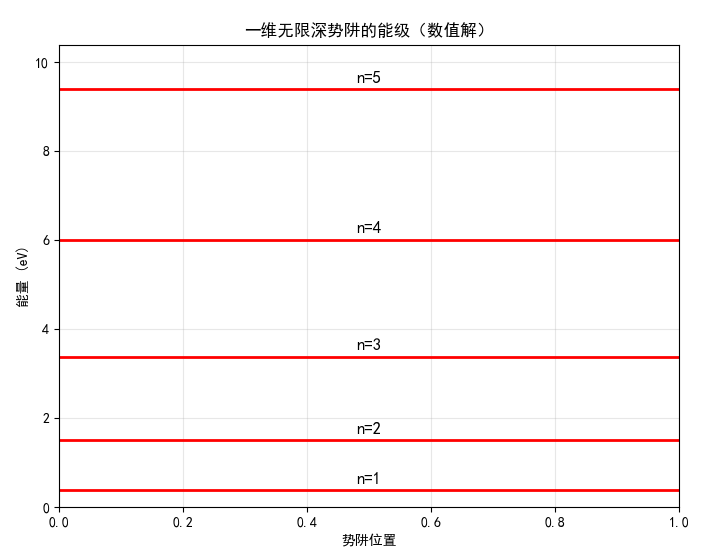
参考资料:
[1] https://ionizing.page/post/schrodinger-equation-numerical-methods/#单粒子定态-schrodinger-方程
【说明:本站主要是个人笔记和代码的分享,内容可能会不定期修改。目前文章支持直接转载,引用或转载请注明出处:https://www.guanjihuan.com 。本站采用知识共享署名许可协议 CC BY】